The degree of a minimal polynomial

Question

Is there in general any way of finding the degree of the factors in the minimal polynomial of an operator without using brute force computation?

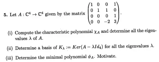
The exercise in question is shown below. It's only this part of (iii) that's bothering me. This is not a homework assignment.

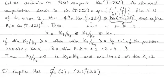
My professor solved this problem for another exercise using the method shown below. I've been trying to understand if this is usable in general and if so how. I tried to adapt the method to this exercise but I didn't arrive at any contradiction.

Answer 1

Suppose $\lambda$ is an eigenvalue of an $n\times n$ matrix $A$ over $\mathbb C$ and let $$ d_i(\lambda)=\dim\ker(A-\lambda I)^i $$ (with $d_0(\lambda)=0$). It's clear that the sequence $d_i(\lambda)$ is nondecreasing. Less obvious is that the successive differences $(d_{i+1}(\lambda)-d_i(\lambda))$ are nonincreasing (this is "(ii) of the previous exercise" in your notes). Since $d_i(\lambda)$ is bounded by $n$, this means $d_i(\lambda)$ is strictly increasing for a while, and then stabilises at some $d(\lambda)$. In fact $d(\lambda)$ is the dimension of the generalized $\lambda$-eigenspace of $A$, and the characteristic polynomial of $A$ is $$ \chi_A(x)=\prod_{\lambda\in\Lambda}(x-\lambda)^{d(\lambda)} $$ where $\Lambda$ is the set of eigenvalues. Let $i(\lambda)$ be the index at which the sequence $d_i(\lambda)$ stabilises, $$ i(\lambda)=\min\{i\mid d_i(\lambda)=d(\lambda)\}. $$ The minimal polynomial of $A$ is $$ \prod_{\lambda\in\Lambda}(x-\lambda)^{i(\lambda)}. $$

---

In the example from your notes, you have $d_1(3)=d(3)=1$ so $i(3)=1$. Also $d_1(2)=2$ and $d(2)=3$. This leaves only one possibility for the sequence $d_i(2)$, namely: $$ (d_0(2),d_1(2),d_2(2),d_3(2),\ldots)=(0,2,3,3,\ldots). $$ Note that the sequence can't be $0,2,2,3,\ldots$ because the successive differences must be nonincreasing. Thus $i(2)=2$. This same reasoning should apply to your exercise.

---

In general $d_1(\lambda)$ and $d(\lambda)$ may not be sufficient to determine $i(\lambda)$. It's possible to compute $\ker(A-\lambda I)^i$ for successive value of $i$ until the dimension stops increasing.

Answer 2

Here's another approach, not sure if compatible with what you've learned so far. If not maybe you can look back later.

You will need Cayley-Hamilton theorem and maybe something more. Background: The minimal polynomial divides the characteristic polynomial.

Cayley-Hamilton theorem is the result that every matrix fulfils it's own characteristic polynomial. Then the factors of the minimal polynomial is a subset of the factors in the characteristic polynomial. In fact it is the minimal degree polynomial ( therefore the name, I'd guess ) that fulfills the equation.

Knowing this we can calculate the vectorization of the first few $A^k$ and then solve an equation system where we equal it to the vectorization of the unit matrix. The lowest possible such $k$ that gives 0 error will have the coefficients of our minimal polynomial! In GNU Octave or matlab this would do:

c = [vec(A),vec(A^2)]\vec(eye(4)); % first try, we know that it needs to be 
%  degree >= 2 because otherwise A would be 0 or a multiple of I, which it isn't.

Subsequent trials would correspond to successively adding a new column $\text{vec}(A^k)$ until

 sum(abs([vec(A),vec(A^2)]*c-vec(eye(4))))

or some other error measure becomes sufficiently small with regard to our numerical precision.

Note that we don't need to find any eigenvalues or multiply together stuff or factor anything. Just a few matrix multiplications followed by linear regression.