NOTE: This answer assumes the heights are normally distributed.
I thought there'd be a well-known distribution for the maximum of n
standard normal variables, but, as
Expected value for maximum of n normal random variable notes, there isn't. You
can't even find a closed form for the mean/expected value (though you can
for the median).
In Mathematica, this distribution is:
"OrderDistribution[{NormalDistribution[0, 1], n}, n]"
The PDF for the max of n standard normal variables is:
$
\frac{2^{\frac{1}{2}-n} n e^{-\frac{x^2}{2}}
\left(\text{erf}\left(\frac{x}{\sqrt{2}}\right)+1\right)^{n-1}}{\sqrt{\pi }}
$
and the CDF is:
$2^{-n} \left(\text{erf}\left(\frac{x}{\sqrt{2}}\right)+1\right)^n$
Here's what the PDF looks like for various values of n:
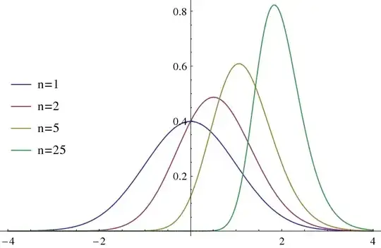
Of course, n=1 is just the standard normal distribution itself.
Except for n=1, these aren't normal distributions, but can be
approximated as such. For n=5, for example,
$\{\mu \to 1.11241,\sigma \to 0.656668\}$ and the graph looks like this:
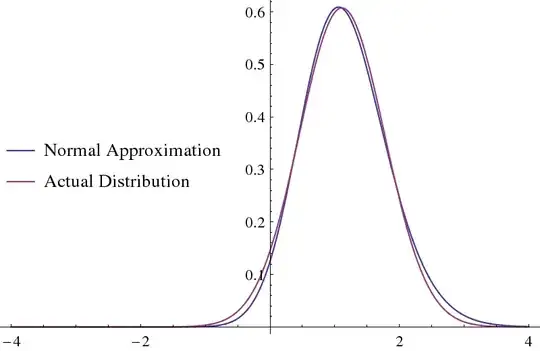
The integral of the difference squared from $-\infty$ to $\infty$ is
about 0.000848615
For n=25, $\{\mu \to 1.89997,\sigma \to 0.486849\}$:
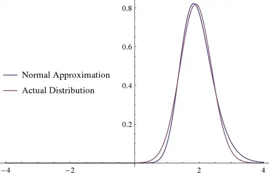
with an error squared of 0.00331485.
In both cases, I used numerical methods to minimize integral of the
difference squared (ie, the "error" squared).
Of course, you used 5 and 25 as examples. Below is a tabulation for
the best fit parameters from 1 to 25, plus some larger values for
comparison (n=1 is the standard normal distribution):
$
\begin{array}{ccccc}
\text{n} & \mu _{\text{fit}} & \sigma _{\text{fit}} & \text{err}^2 & \text{}
\\
1 & 0 & 1 & 0 & \text{} \\
2 & \text{ 0.536} & \text{ 0.820} & \text{ 0.000145} & \text{} \\
3 & \text{ 0.806} & \text{ 0.740} & \text{ 0.000382} & \text{} \\
4 & \text{ 0.983} & \text{ 0.691} & \text{ 0.000622} & \text{} \\
5 & \text{ 1.112} & \text{ 0.657} & \text{ 0.000849} & \text{} \\
6 & \text{ 1.214} & \text{ 0.631} & \text{ 0.001058} & \text{} \\
7 & \text{ 1.297} & \text{ 0.611} & \text{ 0.001252} & \text{} \\
8 & \text{ 1.366} & \text{ 0.595} & \text{ 0.001432} & \text{} \\
9 & \text{ 1.427} & \text{ 0.582} & \text{ 0.001599} & \text{} \\
10 & \text{ 1.479} & \text{ 0.570} & \text{ 0.001755} & \text{} \\
11 & \text{ 1.526} & \text{ 0.560} & \text{ 0.001901} & \text{} \\
12 & \text{ 1.568} & \text{ 0.551} & \text{ 0.002038} & \text{} \\
13 & \text{ 1.606} & \text{ 0.543} & \text{ 0.002167} & \text{} \\
14 & \text{ 1.641} & \text{ 0.536} & \text{ 0.002289} & \text{} \\
15 & \text{ 1.673} & \text{ 0.529} & \text{ 0.002405} & \text{} \\
16 & \text{ 1.703} & \text{ 0.524} & \text{ 0.002515} & \text{} \\
17 & \text{ 1.730} & \text{ 0.518} & \text{ 0.002619} & \text{} \\
18 & \text{ 1.756} & \text{ 0.513} & \text{ 0.002719} & \text{} \\
19 & \text{ 1.780} & \text{ 0.509} & \text{ 0.002815} & \text{} \\
20 & \text{ 1.803} & \text{ 0.504} & \text{ 0.002907} & \text{} \\
21 & \text{ 1.825} & \text{ 0.500} & \text{ 0.002995} & \text{} \\
22 & \text{ 1.845} & \text{ 0.497} & \text{ 0.003079} & \text{} \\
23 & \text{ 1.864} & \text{ 0.493} & \text{ 0.003161} & \text{} \\
24 & \text{ 1.882} & \text{ 0.490} & \text{ 0.003239} & \text{} \\
25 & \text{ 1.900} & \text{ 0.487} & \text{ 0.003315} & \text{} \\
50 & \text{ 2.182} & \text{ 0.440} & \text{ 0.004654} & \text{} \\
100 & \text{ 2.440} & \text{ 0.403} & \text{ 0.006047} & \text{} \\
500 & \text{ 2.971} & \text{ 0.342} & \text{ 0.009231} & \text{} \\
1000 & \text{ 3.176} & \text{ 0.323} & \text{ 0.010527} & \text{} \\
5000 & \text{ 3.616} & \text{ 0.287} & \text{ 0.013320} & \text{} \\
10000 & \text{ 3.791} & \text{ 0.275} & \text{ 0.014434} & \text{} \\
100000 & \text{ 4.328} & \text{ 0.244} & \text{ 0.017810} & \text{} \\
\end{array}
$
I couldn't get Mathematica to compute best fit mean and sd for values
much higher than n=100000, but I didn't try that hard.
I couldn't find a closed form for the best fit mean, or even the true
mean, but there is one for the median:
$\sqrt{2} \text{erf}^{-1}\left(2^{\frac{n-1}{n}}-1\right)$
Since we know the PDF, you'd think we could find a closed form for the
mode, by setting the PDF's derivative to 0, which would be:
$
\frac{2^{-n} e^{-x^2}
\left(\text{erf}\left(\frac{x}{\sqrt{2}}\right)+1\right)^{n-2} \left(\sqrt{2
\pi } n e^{\frac{x^2}{2}} x
\left(\text{erfc}\left(\frac{x}{\sqrt{2}}\right)-2\right)+2 (n-1)
n\right)}{\pi }=0
$
As it turns out
(https://mathematica.stackexchange.com/questions/110564/) this can be
solved for n, but not for x. Thus, I use numerical techniques to
obtain that as well.
Below are the various "means" (including the best-fit mean above) for
various values.
$
\begin{array}{ccccc}
\text{n} & \mu _{\text{fit}} & \mu _{\text{true}} & \text{Median} &
\text{Mode} \\
1 & 0 & 0 & 0 & 0 \\
2 & \text{ 0.536} & \text{ 0.564} & \text{ 0.545} & \text{ 0.506} \\
3 & \text{ 0.806} & \text{ 0.846} & \text{ 0.819} & \text{ 0.765} \\
4 & \text{ 0.983} & \text{ 1.029} & \text{ 0.998} & \text{ 0.936} \\
5 & \text{ 1.112} & \text{ 1.163} & \text{ 1.129} & \text{ 1.062} \\
6 & \text{ 1.214} & \text{ 1.267} & \text{ 1.231} & \text{ 1.160} \\
7 & \text{ 1.297} & \text{ 1.352} & \text{ 1.315} & \text{ 1.241} \\
8 & \text{ 1.366} & \text{ 1.424} & \text{ 1.385} & \text{ 1.309} \\
9 & \text{ 1.427} & \text{ 1.485} & \text{ 1.446} & \text{ 1.368} \\
10 & \text{ 1.479} & \text{ 1.539} & \text{ 1.499} & \text{ 1.420} \\
11 & \text{ 1.526} & \text{ 1.586} & \text{ 1.546} & \text{ 1.466} \\
12 & \text{ 1.568} & \text{ 1.629} & \text{ 1.588} & \text{ 1.508} \\
13 & \text{ 1.606} & \text{ 1.668} & \text{ 1.626} & \text{ 1.545} \\
14 & \text{ 1.641} & \text{ 1.703} & \text{ 1.662} & \text{ 1.580} \\
15 & \text{ 1.673} & \text{ 1.736} & \text{ 1.694} & \text{ 1.611} \\
16 & \text{ 1.703} & \text{ 1.766} & \text{ 1.724} & \text{ 1.641} \\
17 & \text{ 1.730} & \text{ 1.794} & \text{ 1.751} & \text{ 1.668} \\
18 & \text{ 1.756} & \text{ 1.820} & \text{ 1.777} & \text{ 1.693} \\
19 & \text{ 1.780} & \text{ 1.844} & \text{ 1.801} & \text{ 1.717} \\
20 & \text{ 1.803} & \text{ 1.867} & \text{ 1.824} & \text{ 1.740} \\
21 & \text{ 1.825} & \text{ 1.889} & \text{ 1.846} & \text{ 1.761} \\
22 & \text{ 1.845} & \text{ 1.910} & \text{ 1.866} & \text{ 1.781} \\
23 & \text{ 1.864} & \text{ 1.929} & \text{ 1.885} & \text{ 1.800} \\
24 & \text{ 1.882} & \text{ 1.948} & \text{ 1.904} & \text{ 1.819} \\
25 & \text{ 1.900} & \text{ 1.965} & \text{ 1.921} & \text{ 1.836} \\
50 & \text{ 2.182} & \text{ 2.249} & \text{ 2.204} & \text{ 2.117} \\
100 & \text{ 2.440} & \text{ 2.508} & \text{ 2.462} & \text{ 2.375} \\
500 & \text{ 2.971} & \text{ 3.037} & \text{ 2.992} & \text{ 2.908} \\
1000 & \text{ 3.176} & \text{ 3.241} & \text{ 3.198} & \text{ 3.115} \\
5000 & \text{ 3.616} & \text{ 3.678} & \text{ 3.636} & \text{ 3.558} \\
10000 & \text{ 3.791} & \text{ 3.852} & \text{ 3.811} & \text{ 3.735} \\
100000 & \text{ 4.328} & \text{ 4.384} & \text{ 4.346} & \text{ 4.276} \\
\end{array}
$
Of course, if these were true normal distributions, the median, mode,
mean, and "best fit $\mu$" would be identical.
You can estimate the standard deviation by comparing the distribution
to the normal distribution in the limiting case around the
median. This is only estimate I could find with a closed form:
$
\frac{2^{\frac{n-1}{n}}
e^{\text{erf}^{-1}\left(2^{\frac{n-1}{n}}-1\right)^2}}{n}
$
Below is a table of the best fit standard deviation, the true standard
deviation (computed numerically), and the closed-form estimated
standard deviation above:
$
\begin{array}{cccc}
\text{n} & \sigma _{\text{fit}} & \sigma _{\text{true}} & \sigma
_{\text{est}} \\
1 & 1 & 1 & 1 \\
2 & \text{ 0.820} & \text{ 0.826} & \text{ 0.820} \\
3 & \text{ 0.740} & \text{ 0.748} & \text{ 0.740} \\
4 & \text{ 0.691} & \text{ 0.701} & \text{ 0.692} \\
5 & \text{ 0.657} & \text{ 0.669} & \text{ 0.659} \\
6 & \text{ 0.631} & \text{ 0.645} & \text{ 0.634} \\
7 & \text{ 0.611} & \text{ 0.626} & \text{ 0.614} \\
8 & \text{ 0.595} & \text{ 0.611} & \text{ 0.598} \\
9 & \text{ 0.582} & \text{ 0.598} & \text{ 0.585} \\
10 & \text{ 0.570} & \text{ 0.587} & \text{ 0.574} \\
11 & \text{ 0.560} & \text{ 0.577} & \text{ 0.564} \\
12 & \text{ 0.551} & \text{ 0.569} & \text{ 0.555} \\
13 & \text{ 0.543} & \text{ 0.561} & \text{ 0.548} \\
14 & \text{ 0.536} & \text{ 0.555} & \text{ 0.541} \\
15 & \text{ 0.529} & \text{ 0.549} & \text{ 0.534} \\
16 & \text{ 0.524} & \text{ 0.543} & \text{ 0.529} \\
17 & \text{ 0.518} & \text{ 0.538} & \text{ 0.523} \\
18 & \text{ 0.513} & \text{ 0.533} & \text{ 0.519} \\
19 & \text{ 0.509} & \text{ 0.529} & \text{ 0.514} \\
20 & \text{ 0.504} & \text{ 0.525} & \text{ 0.510} \\
21 & \text{ 0.500} & \text{ 0.521} & \text{ 0.506} \\
22 & \text{ 0.497} & \text{ 0.518} & \text{ 0.502} \\
23 & \text{ 0.493} & \text{ 0.514} & \text{ 0.499} \\
24 & \text{ 0.490} & \text{ 0.511} & \text{ 0.496} \\
25 & \text{ 0.487} & \text{ 0.508} & \text{ 0.493} \\
50 & \text{ 0.440} & \text{ 0.464} & \text{ 0.447} \\
100 & \text{ 0.403} & \text{ 0.429} & \text{ 0.411} \\
500 & \text{ 0.342} & \text{ 0.370} & \text{ 0.351} \\
1000 & \text{ 0.323} & \text{ 0.351} & \text{ 0.332} \\
5000 & \text{ 0.287} & \text{ 0.316} & \text{ 0.297} \\
10000 & \text{ 0.275} & \text{ 0.304} & \text{ 0.285} \\
100000 & \text{ 0.244} & \text{ 0.272} & \text{ 0.253} \\
\end{array}
$
As you can see, you can kinda-sorta estimate the best fit mean and
standard deviation based on the closed forms we found earlier.
If we use the best fit approximations, your distributions are:
tallest of 5 from Country A: $\{\mu \to 78.6745,\text{sd}\to 3.94001\}$
tallest of 25 from Country B: $\{\mu \to 71.6999,\text{sd}\to 1.46055\}$
The difference: $\{\mu \to 6.9746,\sigma \to 4.20201\}$ (based on addition of variances)
So the chance A will be taller is about 95.15%
Of course, that's just an approximation, so let's do a more rigorous
analysis below.
The CDF for the tallest of 25 from Country B:
$
\frac{\left(\text{erf}\left(\frac{x-66}{3
\sqrt{2}}\right)+1\right)^{25}}{33554432}
$
and the PDF for the tallest of 5 from Country A:
$
\frac{5 e^{-\frac{1}{72} (x-72)^2} \left(\text{erf}\left(\frac{x-72}{6
\sqrt{2}}\right)+1\right)^4}{96 \sqrt{2 \pi }}
$
If we use Mathematica to numerically integrate the product from
$-\infty$ to $\infty$ we get 95.77%, which is pretty close to our
earlier estimate.
Just for fun, I ran a Monte Carlo simulation as well:
countryA := Max[RandomVariate[NormalDistribution[72, 6], 5]]
countryB := Max[RandomVariate[NormalDistribution[66, 3], 25]]
t =Table[countryA>countryB,{i,1,100000}]
and got 95.79% (I ran it several times, 95.79% is the average).
Mathematica derivations/formulas for this answer can be found at:
https://github.com/barrycarter/bcapps/blob/master/STACK/bc-prob-max.m