Before answering to the question I would like to make a prelimirary comment. The significance of the regression depends of several factors among them the scatter of the experimental data, the number of adjustable parameters of the model and others are important.
In the present example of data, the scatter appears rather large. Considering the data represented in logarithmic coordinates, at first sight a linear regression seems already not bad, as shown on the next figure :
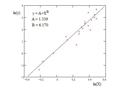
The question is what are the avantage and the drawback to add a adjustable parameter $C$, that is to go from $\quad y=AX^B\quad$ to $\quad y=AX^B+C\quad$ ?
Certainely, if the scatter is not too large, one can expect a better fitting. But if the scatter is large, the improvement of fitting will be not evident : Almost equivalent results will be obtained with a lot of different triplets $(A,B,C)$ which will make doudbtful the significance of the previous parameters $(A,B)$.
This possible drawback must be taken into account. The previous valuable work by Claude Leibovici shows that the confidence intervals on the estimates are large and even more concerning the parameter $B$. This casts a shadow on the ability to obtain significant results.
Nevertheless, even if the available data is not favourable for showing a particular method of regression, the process is presented in full details on the joint page.
The theory can be found in the paper publish on Scribd : https://fr.scribd.com/doc/14674814/Regressions-et-equations-integrales . Page 17 : The practical application to the three parameters power function. The notations are not the same as in the present question. This can be confusing. In order to make it consistent with the notations used here, the notations used in the published paper were changed to write the page below.
The advantage of this method is that it is direct (not iterative) and doesn't require guessed values to start. Of course, if it was really necessary, the estimates obtained could be used as initial values to more advanced methods of non-linear regression.
Note that the order of the data has been changed because it is necessary that the values of $X_k$ be ranked in increassing order.
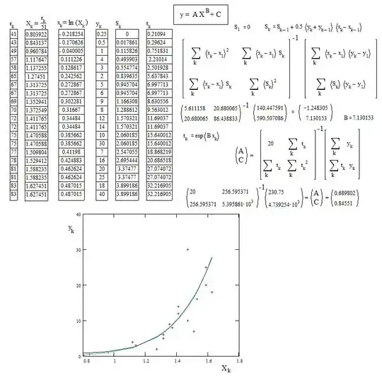
The curve with the estimated parameters is drawn in blue.
As expected, the values $(A,B,C)$ are far from whose already given by Claude Leibovici, but with almost the same result : the coresponding green curve on the figure is quite the same as the blue curve. A difference is only clearly visible at low values of $X$.

