When the population variance is unknown, we should use t-distribution.

Question

It is clear that T-distribution should be used when the sample size is small and the population variance is unknown. My question is Why? Why we use t-distribution in this case? Anybody give me specific reasons for it?

Answer 1

I suppose you have random observations $X_1, X_2, \dots, X_n$ from a population $Norm(\mu, \sigma),$ where both $\mu$ and $\sigma$ are unknown.

Before 1935, when William S. Gossett (writing as 'A. Student'), introduced the t distribution, the practice was to assume $n$ sufficiently large that the sample standard deviation $S$ provides a "good" estimate of $\sigma.$ Then to test $H_O: \mu = \mu_0$ against $H_a: \mu \ne \mu_0$ using the approximate test statistic $$Z_{\text{approx}} = \frac{\bar X - \mu_0}{S/\sqrt{n}}\;\; \text{in place of the exact statistic } Z = \frac{\bar X - \mu_0}{\sigma/\sqrt{n}},$$ rejecting $H_0$ at the 5% significance level when $|Z_{\text{approx}}| > 1.96.$

The contribution of "Student" (with some help from others) was to derive the exact distribution of the statistic $$T = \frac{\bar X - \mu_0}{S/\sqrt{n}},$$ which is now known, and widely tabled, as Student's t distribution with degrees of freedom $\nu = n-1$ or $T(\nu).$

In the technical language of today,

$$T \triangleq \frac{Z}{\sqrt{\chi_{\nu}^2/\nu}},$$

where $Z \sim Norm(0,1)$ and $\chi_{\nu}^2$ is a chi-squared random variable with $\nu$ degrees of freedom.

The critical value of a test at the 5% level is a value $t^*$ that cuts 2.5% of the probability from the upper tail of the distribution $T(\nu)$ and 2.5% of the probability from the lower tail. See below for $\alpha = 5% = 0.05$.

It turns out that $t^* > 1.96$ for all $\nu = n-1,$ but for $n$ larger than about 30, both $1.96$ and $t^*$ round to $2.0.$ Hence the "rule" that "large" samples are those of size greater than 30. (A rule to be used with great caution because it really works only for tests at the 5% level.)

For very small $n,$ it can be disastrous to use $1.96$ instead of $t^*$: for $n = 5,$ we have $t^* = 2.776$. If you were to use $1.96$ instead, the actual rejection rate of $H_0$ would be about 12% instead of the target 5%.

Note: The Wikipedia article on 't distribution' shows plots of the density function of t for several values of $\nu$ and for "$\nu = \infty$," which is standard normal. At the scale of those plots it would be difficult or impossible to distinguish plots of $\nu = \infty$ and $\nu = 50,$ but relative errors in the far tails can be very large.

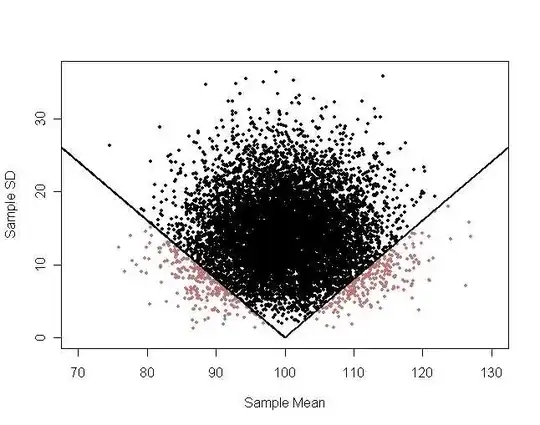
To understand the profound difference between a test using both $\bar X$ and $S$ and a test using only $\bar X$ one can make a bivariate plot or pairs $(\bar X, S)$ from many samples of size five. For these samples $\mu = \mu_0 = 100$ and $\sigma = 15$. In the samples corresponding to light points (5% of them outside the 'envelope flap'), the null hypothesis would be rejected at the 5% level. A test based only on $\bar X$ would have parallel vertical lines as boundaries, ignoring $S$. A t test rejects for the appropriate $combination$ of $\bar X$ far from $\mu_0$ and small $S$.