First, I took some time to verify that the z-test does not
work well when the success probability in the control group
is as small as 10%.
Second, here are some results using a one-sided Fisher's exact test
that rejects the null hypothesis that success probabilities in
the two groups are equal when there are significantly many
more successes is the treatment group than in the control group.
(This means that you would disregard as a fluke any results
with significantly more successes in the control group.)
All of the results below are for Fisher's exact test, and
sample sizes are equal in the two groups. I looked at
cases for $n = n_T = n_C = 50, 100,$ and $200.$
$n = 50.$ Suppose the success probability in the control group is
$\pi_C = 0.02$: If $\pi_T = 0.15,$ then the P-value
averages $.07.$ If $\pi_T = 0.2,$,
the average P-value decreases to $.022.$ And if $\pi_T = 0.25,$
the average p-value decreases to $.007.$ This is summarized
in the first cluster below, and the second cluster is for $\pi_C = 0.1.$
         ppc  ppt   Pv
  n=50   .02  .15  .07
              .20  .022
              .35  .007
         .10  .25  .11     # Scenario (b) below
              .30  .05
              .35  .021    # Scenario (a) below
              .40  .008

  n=100  .02  .10  .06
              .15  .009
              .20  .001
         .10  .20  .10
              .25  .03
              .30  .007

  n=200  .02  .05  .16
              .10  .009
              .15  .0003
         .10  .15  .17
              .20  .028
              .25  .003
              .30  .0002
I hope you can see that this gives you a rough idea what differences
between $\pi_C$ and $\pi_T$ can be reliably detected and at
what level of significance, for each of the three sample sizes.
All average P-value results are based on simulation and are
subject to small simulation errors.
Examples with $n = 100$ and control group with population proportion
of successes $\pi_C = .10$: At the 5% significance level, you will
seldom be able to detect that $\pi_T = .20$ is an improvement,
usually be able to detect that $\pi_T = .25$ is an improvement,
and seldom overlook that $\pi_T = .30$ is an improvement.
If you like, I can show you the R code I used to get these
results. Then you could investigate other scenarios. R is
available free at www.r-project.org and no particular
knowledge of R would be necessary to change numbers in my
program and run additional scenarios.
Finally, I would not trust even Fisher's exact test (any
sample size) unless
the number of successes in the treatment group is at least 5.
Addendum: R code for Fisher exact tests. As requested, here is the R code used to obtain the information
tabled above. Answers for one of the specific tabled situations
is shown. Constants in the first two lines of code may be changed to investigate other situations. (Values for power, included here, are
not tabled above.)
 nc = 50;  nt = 50      # sample sizes
 ppc = .1;  ppt = .35   # population proportions of Success--Scenario (a)
 m = 10^6               # iterations for simulation (adjustable >= 10^4)
 xc = rbinom(m, nc, ppc)   # m-vector of numbers of control Successes
 xt = rbinom(m, nt, ppt)   # m-vector of numbers of treatment Successes
 pv = phyper(xt-1, nt, nc, xt+xc, lower.tail=F)  # m-vect of 1-sided P-vals
 mean(pv)                                        # avg of 1-sided P-vals
 ##  0.02102584
 mean(pv <= .05)  # P(Rej Ho | Ho False as specif) = Power against alt. specif
 ##  0.887290
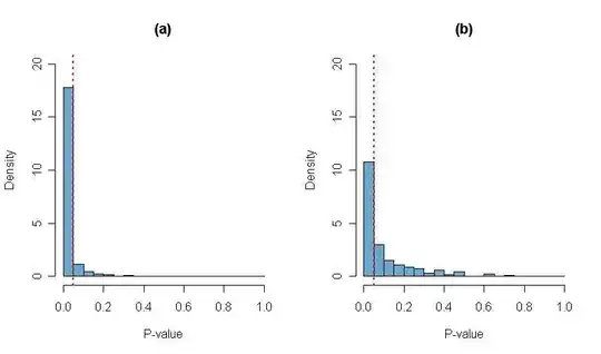
Plots of simulated P-values are shown in the histograms below.
Scenario (a) is for $n_C = n_T = 50;\,
\pi_C = .1, \pi_T = .35$ and in Scenario (b) $\pi_T = .25.$
The vertical dotted red lines are at $0.5,$ so the bar to the
left of the line represents the power of the test, the probability
of rejecting $H_0: \pi_T = \pi_c$ against the alternatives
$H_a: \pi_T > \pi_C$ (as specified), at level $\alpha = 5\%.$
Perhaps the first use of this code should be to verify the values
in the table above to make sure there are no misprints.
