8

As explained here, the average distance or 'travel' of a random walk with $N$ coin tosses approaches: $$\sqrt{\dfrac{2N}{\pi}}$$

What a beautiful result - who would've thought $\pi$ was involved! However, what would be the formula to use for an arbitrary paytable?

For example, a coin toss has the paytable:

  • 0.5 : -1
  • 0.5 : 1

...so a 50% chance of both winning or losing a point. After 10,000 coin tosses, the travel on average will be $\sqrt{10000\cdot2/{\pi}} \approx 79.788$.

However a dice roll where you need to land a six to win could have the paytable:

  • 0.8333.. : -1
  • 0.1666.. : 5

After 10,000 dice rolls, the travel on average will be about 178. However, I only know that because I used simulation to brute force the result - I don't know the formula.

More generally, a paytable could have multiple entries where all the probabilities add up to one:

  • probability1 : payout1
  • probability2 : payout2
  • probability3 : payout3
  • ...
  • ...
  • probabilityN : payoutN

Note that the total of the payouts may not necessarily be zero. It could be weighted to produce an unfair game. For example:

  • 0.75 : -1
  • 0.1 : 0.5
  • 0.15 : 4.5

That's an average payout of $-0.025$ with a variance of $3.811875$, and using simulation, I get $\approx 268.8$ 'travel' from 10000 runs. But how would I find this out directly?

In other words, how would you find the average 'travel' of such a generalized paytable without resorting to simulation? As a side question, would this figure also be a better indication of risk for such a 'game' compared to the standard deviation of the paytable as defined here?

Here's the code I used for the simulation: http://pastebin.com/985eDTFh

It's written in C#, but is otherwise very well self-contained. Most of it is a fast random class, but you can use the default Random class if you prefer. Also, if you're not using C#, don't worry too much about converting the convertCSVtoPayoutTable() function as you can hard code the probability and payout arrays yourself if you prefer.
Dan W
  • 645
  • 1
  • 7
  • 16
  • 3
    In full generality, the asymptotics is $\sqrt{2\sigma^2N/\pi}$ where $\sigma^2$ is the variance of a single step. In your dice example, $\sigma^2=5$ hence, for $N=10'000$, $\sqrt{2\sigma^2N/\pi}=100\sqrt{10/\pi}=178.4124116...$ – Did Aug 17 '15 at 11:26
  • But you have already been explained that, no? – Did Aug 17 '15 at 11:29
  • @Did: Thanks for the feedback. Your formula works for the coin and dice rolls, but when I tried for three entries or more, it differs from the simulation. An example is: probabilities = [0.75, 0.1, 0.15] and payout = [-1, 0.5, 4.5]. That's a variance of 3.811875, but the average 'travel' according to your formula is 155.779 (to 3dp), whilst I get approx 268.8. Could you check your formula? – Dan W Aug 17 '15 at 14:27
  • 1
    Your example is not centered, thus the asymptotics scales like $N$ instead of $\sqrt{N}$, and CLT and variance become irrelevant. – Did Aug 17 '15 at 15:05
  • @Did: Ah, in that case, can you give me the new revised formula which takes into account non-centered paytables? – Dan W Aug 17 '15 at 15:07
  • Sure: if the increments have mean $\mu$, the displacement after $N$ steps is $\mu N+o(N)$ (hence your 268.8 is probably minus 268.8). – Did Aug 17 '15 at 15:11
  • @Did: Can you expand the formula for clarity? I think by a 'mean increment', you're referring to the expected payout (which is $prob_1pay_1 + prob_2pay_2 + prob_3*pay_3$), but I'm not sure how to interpret o(N) from your comment... – Dan W Aug 17 '15 at 15:25
  • In Landau's notation, o(N) is any term negligible with respect to N when N goes to infinity. – Did Aug 17 '15 at 17:42
  • @Did: Had time to revisit this. Assuming N=10000, I'm not sure how to resolve $(0.75-1 + 0.10.5 + 0.15*4.5) + o(10000)$ to equal -268.8. The first part of that sum equals -0.025. The second part (o(N)) from what I understand is the set of functions which have a lower rate of growth than N, so it could be almost anything. Somehow, I'm supposed to ascertain around -269 from that? Perhaps I could open a bounty if the expansion is more complex than I anticipated. – Dan W Sep 16 '15 at 02:07
  • Even the first result that you cite has smaller error terms since it relies on the central limit theorem. – DirkGently Sep 16 '15 at 04:31
  • Thiis is becoming repetitive, but... First, your (0.75∗−1+0.1∗0.5+0.15∗4.5) should read (0.75∗−1+0.1∗0.5+0.15∗4.5)10000. Second, asymptotics are a form of information about, say, a sequence, when $N\to\infty$ only*, hence a term like o(10000) is just absurd. – Did Sep 16 '15 at 05:34
  • @Did: Thanks. Regardless, that still leaves a lot to the imagination with my current level of mathematical knowledge, but I'll open a bounty. – Dan W Sep 16 '15 at 16:44
  • Suppose the jumps $X_1,X_2,\ldots$ are i.i.d. with mean $\mu$ and variance $\sigma^2$. Let $Y_n = |X_1+X_2+\ldots+X_n|$ (the absolute distance traveled after $n$ jumps). If $\mu=0$, then $E[Y_N]\sim \sqrt{2N\sigma^2/\pi}$. If $\mu\neq 0$, then $E[Y_N]\sim \mu N$. That's it. In the $\mu\neq 0$ case, the nonzero mean overwhelms the noise. – mjqxxxx Sep 16 '15 at 19:13
  • @mjqxxxx: Thanks that's clear, but $μN$ would then simply equal -0.025*10000 = -250. But my simulation returns around -268. Do you think my simulation is mistaken? – Dan W Sep 16 '15 at 21:41
  • Just to add I now understand that in the limit where N tends to infinity, $μN$ does indeed equal what I'm after. But not for a finite number such as 10000 runs, so I would like the solution for an arbitrary number of runs. Things are beginning to make a lot more sense now. – Dan W Sep 17 '15 at 00:59
  • @mjqxxxx, you mention that the nonzero mean overwhelms the noise. I have written a new answer below elaborating on this. However, surely there is an explicit formula for the error term, given the value of the non-zero mean, and other parameters such as the variance of a step? If you have time please comment. Thank you. – Colm Bhandal Sep 18 '15 at 20:20

1 Answers1

2

Elaborating on the comments, here is an answer to your question. Basically all the confusion lies in the difference between expected value and expected distance- at least it did for me. For a distribution centred at the origin, this difference is huge, and for large $N$ tends towards:

$$\sqrt{\dfrac{2\sigma^2 N}{\pi}}$$

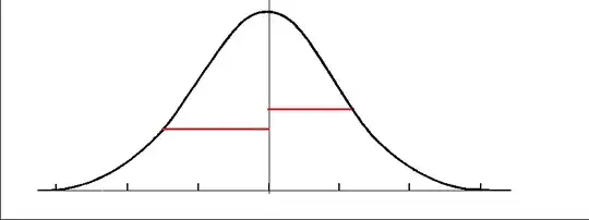
This is clearly a lot bigger than the expected value, which is $0$. This makes sense, intuitively, if you draw out a normal distribution. Note that because you are adding random independent variables with a well-defined mean and variance it's OK to make the assumption of an approximate normal distribution, by the central limit theorem. The approximation gets better with $N$. Now, values cancel out in this normal distribution, leaving a mean of $0$, but distances don't. See the lines in red in the below image- these are distances- they both contribute positively towards expected distance.

Normal centred at 0

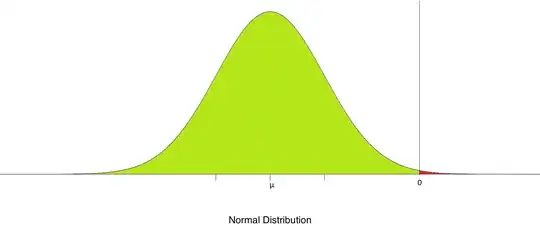
OK, but what if the distribution is shifted? What does this do to the average distance? What it does is it makes it much closer to the average value. The reason is that the further you shift, left or right, the tinier the remainig positive/negative tail becomes. Hence the average distance and the average value tend towards the same thing. See the image below for what I'm talking about. In the calculation for expected value, the red shaded part cancels out its corresponding tail on the other side. In the calculation for expected distance on the other hand, the red shaded part contributes positively towards the total distance. But it's so tiny that the difference is negligible the further the distribution is shifted. This explains the tiny discrepancy between your observed $263$ and the actual mean of $250$. It makes sense: the absolute average distance must be greater than the mean, because there is no "cancelling out" of tails.

Shifted Distribution

To be more formal about the whole thing, let's write some formulas. The expected distance is

$$E(|x|) = \lim_{n\rightarrow\infty}\dfrac{\sum_{i = 1}^n |x_i|}{n}$$

Whereas the expected value is:

$$E(x) = \lim_{n\rightarrow\infty} \dfrac{\sum_{i = 1}^n x_i}{n}$$

Here $x_i$ is just an observation after you run the experiment for the $i^{th}$ time. Also $n$ is the number of experiments. It's different to $N$, the number of steps (dice rolls) per experiment. Now, let Let $U$ be the bag (set with multiplicity) of values $u_i$ in the observed sample set that are positive. And let $V$ be the bag of values $v_i$ that are negative. Then we can also express expected value as follows:

$$E(x) = \lim_{n\rightarrow\infty} \dfrac{\sum_{u_i \in U} |u_i| - \sum_{v_i \in V} |v_i|}{|U| + |V|}$$

Note that $n$ is just the number of experiments/trials and $|U| + |V| = n$. Now, the expected distance is:

$$E(|x|) = \lim_{n\rightarrow\infty} \dfrac{\sum_{u_i \in U} |u_i| + \sum_{v_i \in V} |v_i|}{|U| + |V|}$$

The only difference is a plus sign. Clearly then, as either $U$ or $V$ dominates because of a sliding mean, $E(|x|)$ tends towards $|E(x)|$, with a small error term. The error term will correspond to the leftover (smaller) tail of the distribution on either the positive or negative axis. Without loss of generality, let's say there are more negative than positive values i.e. the positive tail is shorter. Then explicitly, the error term is:

$$E(|x|) - |E(x)| = \lim_{n\rightarrow\infty} \dfrac{2\sum_{u_i \in U} |u_i|}{n}$$

When the mean is $0$, this error term is maximised at:

$$\sqrt{\dfrac{2\sigma^2 N}{\pi}}$$

But as you can see from the shape of the normal curve, it rapidly decreases. This agrees with your observation, with an error term of only around $13$. Of course, I realise that this doesn't answer the question, as I haven't given an explicit formula for the error term! But I believe this answer has enough intuitive value to explain your observed results.

Colm Bhandal
  • 4,649
  • I plugged in the numbers $-0.02510000 + \sqrt{23.811875*10000/\pi}$ but got apx 94 (or -405 if I tried using negative instead of positive between the terms). I expected 268.8 (or -268.8) as I detailed in my question. Where I have gone wrong? I presume $\sigma^2$ = 3.811875. – Dan W Sep 17 '15 at 17:43
  • Maybe you have not gone wrong. Maybe I have gone wrong. I will flag this to the expert Did in the comments above, if he is not too exasperated hopefully he will have an insight. – Colm Bhandal Sep 18 '15 at 10:39
  • After a finite number of runs $N$ the result is random. Loosely speaking, the CLT describes the limit of the probability that this random result $X_N$ is around its expectation $E(X_N)=\mu N$ in the $\sqrt{N}$ scale. More rigorously, consider the event $A_N=[\mu N+a\sqrt{2\sigma^2N/\pi}<X_N<\mu N+b\sqrt{2\sigma^2N/\pi}]$, then the CLT asserts that $P(A_N)$ converges to some $p$ in $(0,1)$ when $N\to\infty$, where $p=P(a<Z<b)$ for some standard normal random variable $Z$. Note that, formally, CLT says nothing about the discrepancy between $P(A_N)$ and $p$ when $N$ is large ... – Did Sep 18 '15 at 10:54
  • ... but that there exists more refined results which guarantee that in the present case, say for $a=-2$ and $b=2$, indeed $P(A_N)$ is close to $p$. Note that here $(a,b)$ are fixed and $N\to\infty$. Note also that CLT says really nothing about the probability that $X_N=\mu N+c\sqrt{2\sigma^2N/\pi}]$ for some fixed $c$, when $N$ is large. Hmmm... Did I just recall some basics about CLT explained everywhere on the internet and in particular on WP? I am afraid I did exactly that. – Did Sep 18 '15 at 10:56
  • @DanW, can you run your simulation for a centred distribution, still using 10,000 steps, and check if even the RHS formula $\sqrt{\dfrac{2\sigma^2 N}{\pi}}$ holds? If it doesn't, then the problem is with that. Else the problem is with this sliding average. – Colm Bhandal Sep 18 '15 at 11:20
  • @DanW my answer was way off. Above is an explanation that I think works. – Colm Bhandal Sep 18 '15 at 20:08
  • Okay, I tried and it passed. My new zero-mean test was 0.75:-1, 0.1:0.75, 0.15:4.5 = 156.233 apx travel in the simulation which closely matches the formula $\sqrt{23.8437510000/pi}=156.4$. Also tried 0.5:-1, 0.25:1, 0.25:1 which comes out the same as the coin-toss paytable 0.5:-1, 0.5:1 (= 78.8 approx) as expected. I'm pretty confident the simulation is accurate. – Dan W Sep 19 '15 at 02:35
  • @DanW your simulation, and the formula, are fine. The above answer shows why the whole thing goes out the window once the mean starts moving. Your best guess in that case is the mean- plus some tiny error term that you get from the two tails of the distribution. – Colm Bhandal Sep 19 '15 at 17:23
  • @ColmBhandal: Thanks, any chance for a closed-form version and/or for a more accurate version that solves the tiny error thing? Also the latter two limit equations use n for the variable towards infinity, but it isn't used. – Dan W Sep 19 '15 at 20:59
  • @DanW I'll work on it. I'm not a statistician (as you can tell) but I find this problem interesting. I'll ask one of my stat friends if I get the chance. The number $n$ is just the number of experiments you do. E.g. the number of times you run your computer simulation. I'm basically taking a frequentist standpoint of the distribution: https://en.wikipedia.org/wiki/Frequentist_probability – Colm Bhandal Sep 21 '15 at 12:04
  • Thanks, great presentation, and probably bounty worthy. The 'tails-not-cancelling' concept made sense too. I'm having a little trouble with interpretation - can you show explicitly plugging in the numbers to the final formula so I can see it more clearly to see how 268.8 is reached (or perhaps rather 18.8 as that's the difference between that and 250). Here they are again: INPUT: outcomesprobability:profit = {0.75:-1, 0.1:0.5, 0.15:4.5}, mean=-0.025, runs=10000. OUTPUT = 268.8. Excuse the more programmer-like description there. Hopefully it's clear. – Dan W Sep 24 '15 at 07:22
  • 1
    @DanW: First of all, this question is not bounty worthy. I didn't answer your question, so I don't get the bounty. Please do not falsely award it to me. Secondly, I am a computer programmer. I asked my stat friend to look at this but she is busy at the moment (PhD woes). As for the formula... I haven't given you a closed form. But if you modify your computer program to count only positive values, then divide by $10000$, you should get $9.4$ (half of $18.8$) according to my non-closed-form formula. I would love to see the result! – Colm Bhandal Sep 24 '15 at 11:53
  • @DanW the modification should be easy: just put one line of code into your program that checks (x > 0) before incrementing the running total (assuming that's how you have things set up) – Colm Bhandal Sep 24 '15 at 11:56
  • Aha, yes I get roughly around 9.38-9.4 after simulating 10M 'universes' (which you call experiments). Let me know if you'd like the code (it's in C# but is easily transferable to other languages). – Dan W Sep 25 '15 at 07:13
  • @DanW FANTASTIC! Great to see experiment agreed with calculation. post your code up to github if you have time and send me link, but dont stress about it! – Colm Bhandal Sep 25 '15 at 12:33
  • 1
    Sure. Here you go: http://pastebin.com/985eDTFh - Don't worry about the size - three quarters of it is code for a fast random class I pinched from Stackoverflow. You can use the default Random class if you prefer. Also, if you're not using C#, don't worry too much about converting the convertCSVtoPayoutTable() function as you can hard code the probability and payout arrays yourself if you prefer. – Dan W Sep 25 '15 at 17:31
  • @DanW that's great. Maybe you could even add the code as an update to the question so that future browser's of the site will see it and it is not lost down here in the murky comments section ;) – Colm Bhandal Sep 28 '15 at 11:56
  • @ColmBhandal: Okay done! – Dan W Sep 29 '15 at 12:04