This is a historical name for the shape parameter of a chi-squared distribution.
Suppose we have a dataset $X_1, \dots, X_n$ from a normal
distribution with unkinown mean $\mu$ and unknown variance $\sigma^2$. Then
then the sample variance is defined as
$S^2 = \frac{\sum_{i=1}^n (X_i - \bar X)^2}{n-1},$ where $\bar X$
is the sample mean. The sample variance is used to
estimate the population variance $\sigma^2.$ In that case $Q = (n-1)S^2/\sigma^2 \sim Chisq(DF = n-1).$
Roughly, the proof begins by regarding the data as a vector in
$n$-dimensional space. The sample mean represents one linear
restriction on the data, leaving $n-1$ dimensions "free" to represent
the variance. The term 'degrees-of-freedom' frequently stands
for dimensionality.
If $\mu$ were known, then the quantity
$V = \frac{\sum_{i=1}^n (X_i - \mu)^2}{n}$ might be used to
estimate the population variance $\sigma ^ 2$.
In this simpler case
$$nV/\sigma^2 = \sum_{i=1}^n \left(\frac{X_i - \mu}{\sigma}\right)^2 = \sum_{i-1}^n Z_i^2 \sim Chisq(DF = n),$$
where the $Z_i$ are iid standard normal. (It is easy to show
with generating functions that the sum of squares of $n$
independent standard normals in chi-squared.)
So one often says that we have "lost one degree of freedom" for estimating $\sigma^2$ because
of the need to estimate $\mu.$
A more elementary (if less complete) explanation is that we divide by $n-1$ in
the definition of $S^2$ because $\sum_{i=1}^n (X_i = \bar X) = 0.$
Hence only $n - 1$ of the deviations $(X_i - \bar X)$ from
the mean are "free" to vary.
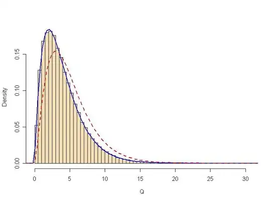
Below is a brief simulation using 100,000 samples of size $n=5$
from the distribution $Norm(\mu=100, \sigma=15).$ It shows that the simulated
distribution of $Q$ is $Chisq(DF = 4)$ [blue density curve] and
not $Chisq(DF = 5)$ [broken red curve].
 m = 10^5;  n = 5;  mu = 100;  sg = 15
 DTA = matrix(rnorm(m*n, mu, sg),nrow=m)  # each row a sample of 5
s.sq = apply(DTA, 1, var)
mean(s.sq)
##  225.123  # sim E(sample var) close to pop var 225
Q = (n-1)*s.sq/sg^2
mean(Q)
##  4.002187 # sim E(Q) close to mean of Chisq(4)