Given the linear system
$$
\mathbf{A} x = y,
$$
the least squares solution is defined as
$$
x_{LS} = \left\{
x \in \mathbb{R}^{n} \colon
\lVert
\mathbf{A} x - y
\rVert_{2}^{2}
\text{ is minimized}
\right\}
$$
Please note that the length $\lVert x \rVert$ is not minimized here. It is the difference between data and prediction $\lVert \mathbf{A}x-y \rVert$ which is minimized.
The general least squares solution is
$$
x_{LS} =
\color{blue}{\mathbf{A}^{+}b} +
\color{red}{\left( \mathbf{I}_{n} - \mathbf{A}^{+}\mathbf{A} \right) z}, \quad z \in \mathbf{R}^{n}
$$
Because you have stipulated an underdetermined problem where $m<n$, the solution will not be unique. The affine space of least squares minimizers is represented by the red dashed line in the figure below.
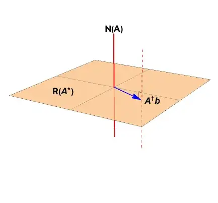
The solution vector of least length is the vector which lies within the column space, $\color{blue}{\mathbf{A}^{+}b}$.
You ask about the projector matrix
$$
\color{red}{\mathbf{P}_{\mathcal{N}(\mathbf{A})}} =
\color{red}{\left( \mathbf{I}_{n} - \mathbf{A}^{+}\mathbf{A} \right)} =
\color{red}{\mathbf{V}_{\mathcal{N}} \mathbf{V}_{\mathcal{N}}^{*}}
$$
which assume the singular value decomposition
$$
\begin{align}
\mathbf{A} &=
\mathbf{U} \, \Sigma \, \mathbf{V}^{*} \\
%
&=
% U
\left[ \begin{array}{cc}
\color{blue}{\mathbf{U}_{\mathcal{R}}} & \color{red}{\mathbf{U}_{\mathcal{N}}}
\end{array} \right]
% Sigma
\left[ \begin{array}{cccccc}
\sigma_{1} & 0 & \dots & & & \dots & 0 \\
0 & \sigma_{2} \\
\vdots && \ddots \\
& & & \sigma_{\rho} \\
& & & & 0 & \\
\vdots &&&&&\ddots \\
0 & & & & & & 0 \\
\end{array} \right]
% V
\left[ \begin{array}{c}
\color{blue}{\mathbf{V}_{\mathcal{R}}}^{*} \\
\color{red}{\mathbf{V}_{\mathcal{N}}}^{*}
\end{array} \right] \\
%
& =
% U
\left[ \begin{array}{cccccccc}
\color{blue}{u_{1}} & \dots & \color{blue}{u_{\rho}} & \color{red}{u_{\rho+1}} & \dots & \color{red}{u_{n}}
\end{array} \right]
% Sigma
\left[ \begin{array}{cc}
\mathbf{S}_{\rho\times \rho} & \mathbf{0} \\
\mathbf{0} & \mathbf{0}
\end{array} \right]
% V
\left[ \begin{array}{c}
\color{blue}{v_{1}^{*}} \\
\vdots \\
\color{blue}{v_{\rho}^{*}} \\
\color{red}{v_{\rho+1}^{*}} \\
\vdots \\
\color{red}{v_{n}^{*}}
\end{array} \right]
%
\end{align}
$$
Constructing the Moore-Penrose pseudoinverse
$$
\mathbf{A}^{+} =
\left[ \begin{array}{cc}
\color{blue}{\mathbf{V}_{\mathcal{R}}} & \color{red}{\mathbf{V}_{\mathcal{N}}}
\end{array} \right]
%
\left[ \begin{array}{cc}
\mathbf{S}^{-1} & \mathbf{0} \\
\mathbf{0} & \mathbf{0}
\end{array} \right]
%
\left[ \begin{array}{c}
\color{blue}{\mathbf{U}^{*}_{\mathcal{R}}} \\ \color{red}{\mathbf{U}^{*}_{\mathcal{N}}}
\end{array} \right]
$$
leads to
$$
\mathbf{A}^{+} \mathbf{A} =
%
\left[ \begin{array}{cc}
\color{blue}{\mathbf{V}_{\mathcal{R}}} & \color{red}{\mathbf{V}_{\mathcal{N}}}
\end{array} \right]
%
\left[ \begin{array}{cc}
\mathbf{I}_{\rho} & \mathbf{0} \\
\mathbf{0} & \mathbf{0}
\end{array} \right]
%
\left[ \begin{array}{c}
\color{blue}{\mathbf{V}^{*}_{\mathcal{R}}} \\ \color{red}{\mathbf{V}^{*}_{\mathcal{N}}}
\end{array} \right]
$$
You can see how the central matrix product acts like a stencil, removing all range space components.
