Impact of random numbers on the eigen-values

Question

How do the eigen-values of the following tridiagonal matrix ($A$) change when adding random numbers $R_i$ (with a normal distribution with the mean 0 and variance $m$) to its diagonal. A is a square matrix defined as follows:

For i = 1 to N $$ A(i,i) = -2 + R_i $$ $$ A(i,i+1) = 1 $$ $$ A(i,i-1) = 1 $$ where m and N are constants.

Notice that the eigen-values are known for the case $R_i=0$:

for j=1 to N; $$ Eig(j) = -2 -2 cos(j\pi/N) $$

Numerical solution reveals that the eigen values around the maximum eigenvalue have the largest deviation from the case without random numbers ($R_i=0$). For example, the following figure shows eigen values with and without having the random numbers for m=0.1. But how we can solve the problem analytically? (Maybe by using central limit theorem)

Answer 1

I don't think this question has an easy answer. See section 1.3, "Eigenvalues and sums of Hermitian matrices," of Terry Tao's book on random matrices.

Answer 2

This seems to fall under eigenvalue perturbation problem.

The following assumes that eigenvectors $x_{0j}$ of the unperturbed matrix are chosen such that $||x_{0j}||^2 = x_{0j}^{*} x_{0j} = 1$.

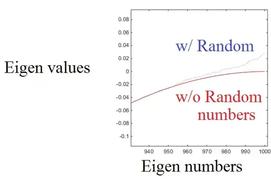
An eigenvalue of perturbed matrix is $\lambda_j = \lambda_{0j} + \mathbf{x}_{0j}^{*} \delta A \mathbf{x}_{0j} + o(||\delta A||)$, where $\lambda_{0j} = -2 - 2 \cos (2 \pi j/N)$ is $j$-th eigenvalue for unperturbed matrix, $\mathbf{x}_{0j}$ is the corresponding eigenvector and $\delta A$ is a diagonal matrix with $R_i$ on its diagonal, $||\delta A|| = \max |R(i)|$. As a result, up to higher-degree , the expectation of $\lambda_j$ is the non-perturbed value $\lambda_{0j}$ and, if $R_i$ are uncorrelated, then $$ \mathrm{Var}(\lambda_j) = \mathrm{Var} \left(\sum_{k=1}^N R_k |(x_{0j})_k|^2 \right)= \sum_{k=1}^N \mathrm{Var} (R_k |(x_{0j})_k|^2) = \sum_{k=1}^N |(x_{0j})_k|^4 m \leq m $$ (up to higher-degree terms). Since eigenvectors have the form $(x_{0j})_k = \sqrt{1/N}\exp(-i t_{jk})$ with real $t_{jk}$, $|(x_{0j})_k|^2 = 1/\sqrt{N}$ for all $k$ and thus, $\lambda_j = \lambda_{0 j} + \frac{1}{N} \sum_{k=1}^N R_k + o(||\delta A||)$ and $\mathrm{Var}(\lambda_j) = m/N$.

For reference, the second-order and third-order corrections are $$ \delta \lambda^{(2)} = \sum_{\substack{k=1\\ k \neq j}}^{N} \frac{|x_{0k}^{*} \delta A x_{0j}|^2}{\lambda_{0j} - \lambda_{0k}} $$ and $$ \delta \lambda^{(3)} = \sum_{\substack{k=1\\ k \neq j}}^{N} \sum_{\substack{m=1\\ m \neq j}}^{N} \frac{x_{0j}^{*} \delta A x_{0m} x_{0m}^{*} \delta A x_{0k} x_{0k}^{*} \delta A x_{0j}}{(\lambda_{0m} - \lambda_{0j})(\lambda_{0k} - \lambda_{0j})} - x_{0j}^{*} \delta A x_{0j} \sum_{\substack{m = 1\\m \neq j}} \frac{|x_{0j}^{*} \delta A x_{0m}|^2}{(\lambda_{0m} - \lambda_{0j})^2}. $$

The formula for mean value for $\max R_i$, which describes how accurate above estimations are, can be found in Expectation of the maximum of gaussian random variables.

As a result of Bauer–Fike theorem, for any eigenvalue of the perturbed matrix $\lambda$ there is an eigenvalue of unperturbed matrix $\lambda_0$ such that $|\lambda - \lambda_0| \leq \max R_i$.

In addition, it follows from Gershgorin circle theorem that all eigenvalues belong to $[-4, 0]$.