Can it be shown that $Y_0(\lambda_n a)J_0(\lambda_n a) - J_0(\lambda_n a)Y_0(\lambda_n a) \ne 0$?

Question

Background

I am currently looking into the task of describing a transient temperature field $\theta(r,t)$ across the thickness $a \leq r \leq b$ of an infinitely long and hollow cylinder exposed to a sinusoidal temperature signal applied at the inner boundary $g(t)=\theta_0 \sin(2\pi \cdot f \cdot t)$.

The following thermal boundary conditions apply

$\theta(a,t)=g(t)$ $\quad$ for $t\ge0$, $\quad$ (1)

$\theta(b,t)=0$ $\quad$ for $t\ge0$, $\quad$ (2)

$\theta(r,0)=0$. $\quad$ (3)

The starting point for the derivation is the heat diffusion equation ($\alpha^*$ is the thermal diffusivity) in cylindrical coordinates

$\frac{\partial^2\theta}{\partial r^2} + \frac{1}{r}\frac{\partial\theta}{\partial r} = \frac{1}{\alpha^*}\frac{\partial\theta}{\partial t}$. $\quad$ (4)

The derivation of the final expression (which applies the Hankel transform followed by the inverse transform) for the temperature distribution can be found in several papers, for example [Shahani A.R. and Nabavi S.M. (2007) Applied Mathematical Modelling, Vol 31, p 1807-1818]. The final expression reads

$\theta(r,t)=-\alpha^*\pi \sum\limits_{n=1}^\infty \frac{\lambda^2_n J^2_0(\lambda_n b)}{J^2_0(\lambda_n a)-J^2_0(\lambda b)} \left[ Y_0(\lambda_n a)J_0(\lambda_n r) - J_0(\lambda_n a)Y_0(\lambda_n r) \right]\left[ e^{-\alpha^*\lambda_n^2 t} \int_0^t e^{\alpha^*\lambda_n^2\tau} g(\tau) d\tau \right]$ $\quad$ (5)

where $\lambda_n$ are the positive roots of the transcendental equation

$Y_0(\lambda_n a)J_0(\lambda_n b) - J_0(\lambda_n a)Y_0(\lambda_n b) = 0$ $\quad$ (6)

and $J_0(z)$ and $Y_0(z)$ are Bessel functions of order $0$ of the first and second kind, respectively.

Result

I have managed to implement the required code (as I understand it) in Matlab. The literature states that 100 roots is sufficient. When I plot the temperature field versus the thickness I get a strange temperature distribution for cases other than $g(t)=0$ as shown by the figure below (the blue and green curves are correct while the black and red curves are not).

enter image description here

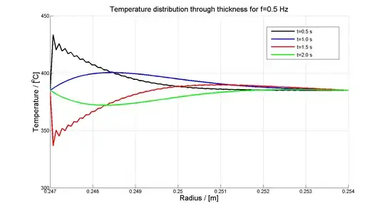
My implementation does not seem to fulfill the boundary condition (1) which is also indicated by oscillations for the remainder of the corresponding (black and red) curves. My math skills are unfortunately rather limited and I do not seem to be able to see how the final expression (5) fulfills the boundary condition (1).

Question

Can it be shown that $Y_0(\lambda_n a)J_0(\lambda_n a) - J_0(\lambda_n a)Y_0(\lambda_n a) \ne 0$? Is this where my implementation goes wrong or is my mistake perhaps to be found elsewhere?

You can try posting a link to the graph you have, and somebody will embed the image for you... — J. M. ain't a mathematician, Apr 18 '12 at 16:11
@J.M.: I managed to upload the image myself thanks to increased reputation. — Daniel Bremberg, Apr 18 '12 at 16:53
Umm, $Y_0(\lambda_n a) J_0(\lambda_n a) - J_0(\lambda_n a) Y_0(\lambda_n a) = 0$ by the commutative law of multiplication. Or did you mean something else? — Robert Israel, May 21 '12 at 17:28
I'm a little confused, because the form of the question at the end of the Q (and the one in the title) has an expression that's trivially zero; should some of those $a$s be $b$s (or possibly $r$s)? — Steven Stadnicki, May 21 '12 at 17:29
@RobertIsrael Of course it is a typo, Daniel surely means the expression in the sum of (5) where thus it should be $r$ instead of two instances of $a$. — AD - Stop Putin -, Sep 28 '12 at 14:13

score 0 · Answer 1 · edited Jun 27 '12 at 12:07

Plot roots of Eq.(6) which you insert in Eq.(5) - do you separate negative and positive ones correctly?
Check your code for the case $g(t)=$ const. Does it work?
Why do you think that the blue and green curves are correct, if they have a non-zero asymptote towards $r=b$? (so Eq.(2) is not fulfilled)
Answer to the question: if you have derived a root for Eq.(6), and insert it back into this equation, you'll always get zero :-)

Best regards, Vitaly.

P.S.: I think, you can simplify your Matlab code, since Exp*Sin can easily be integrated. Maybe you have already implemented this but just in case:

Int(Exp(m*t)*Sin(n*t))dx = (Exp(m*t))*(m*Sin(n*t) - n*Cos(n*t))/(m^2 + n^2)

Can it be shown that $Y_0(\lambda_n a)J_0(\lambda_n a) - J_0(\lambda_n a)Y_0(\lambda_n a) \ne 0$?

1 Answers1