gaussian integral of power of cdf : $\int_{-\infty}^{+\infty} \Phi(x)^n \cdot \phi(a+bx) \cdot dx$

Question

Is there an analytic solution for the following Gaussian integral?

$$\int_{-\infty}^{+\infty} \Phi(x)^n \cdot \phi(a+bx) \cdot dx$$

with

• $n$, a positive integer (typically under 10)
• $a,b$, real numbers (typical values: $a$ between 1 and 30, and $b$ between 1 and 10)
• $\Phi(\cdot)$, the standard normal cumulative distribution function
• $\phi(\cdot)$, the standard normal density function

I found a solution for $n=1$ and $n=2$ (see http://en.wikipedia.org/wiki/List_of_integrals_of_Gaussian_functions)

However, I would need a general solution (for any $n$) if it exists. If not, is there a good approximation?

Thanks.

Answer 1

Let us denote the following. \begin{eqnarray} {\mathfrak J}^{(n)}(a,b)&:=&\int\limits_{\mathbb R} [\Phi(x)]^n \cdot \phi(a+b x) dx\\ &=& \int\limits_{\mathbb R} [\Phi(\frac{x-a}{b})]^n \cdot \phi(x) \frac{dx}{b} \end{eqnarray} Now, by differentiating the lower equality with respect to $a$ and then by completing to square the resulting Gaussian functions in the integrand we easily establish the following recurrence relation: \begin{equation} \partial_a {\mathfrak J}^{(n)}(a,b) = (-n) \frac{\phi(\frac{a} {\sqrt{1+b^2}})}{b} {\mathfrak J}^{(n-1)}\left( \frac{a b}{\sqrt{1+b^2}},\sqrt{1+b^2}\right) \end{equation} for $n=1,2,3,\cdots$ subject to the initial condition: \begin{equation} {\mathfrak J}^{(0)}(a,b)=\frac{1}{b} \end{equation} and the boundary condition ${\mathfrak J}^{(n)}(\infty,b)=0$.

Hence we have: \begin{eqnarray} {\mathfrak J}^{(1)}(a,b)&=& \frac{1}{b} \left(1-\Phi(\frac{a}{\sqrt{1+b^2}})\right)\\ {\mathfrak J}^{(2)}(a,b)&=& \frac{1}{b} \left(1-\Phi(\frac{a}{\sqrt{1+b^2}})\right)- \frac{2}{b} T\left(\frac{a}{\sqrt{1+b^2}},\frac{b}{\sqrt{2+b^2}}\right)\\ {\mathfrak J}^{(3)}(a,b)&=& \frac{3}{2 b} \left(1-\Phi(\frac{a}{\sqrt{1+b^2}})\right)-\frac{3}{b} T\left(\frac{a}{\sqrt{1+b^2}},\frac{b}{\sqrt{2+b^2}}\right)-\\ &&\frac{6}{b} \int\limits_{\frac{a}{\sqrt{1+b^2}}} \phi(\xi) T\left(\xi \frac{b}{\sqrt{2+b^2}},\frac{\sqrt{1+b^2}}{\sqrt{3+b^2}} \right) d\xi\\ &=&\frac{1}{b} + \sqrt{2} a \phi(\frac{\sqrt{2} a}{\sqrt{2+b^2}}) \cdot \frac{\left(-\sqrt{2} \sqrt{\frac{b^2+1}{b^2+2}}-\frac{6 \arctan\left(\sqrt{\frac{b^2+3}{b^2+1}}\right)}{\pi }+3 \right)}{2 \sqrt{2} b \sqrt{b^2+1}}+\\ &&-\frac{3}{2 b} \Phi(\frac{a}{\sqrt{1+b^2}})+\frac{1}{2 b} \Phi(\frac{\sqrt{2} a}{\sqrt{2+b^2}})-\frac{3}{b} T\left(\frac{a}{\sqrt{1+b^2}},\frac{b}{\sqrt{2+b^2}}\right)\\ {\mathfrak J}^{(4)}(a,b)&=& \frac{1}{b} + \sqrt{2} a \phi(\frac{\sqrt{2}a}{\sqrt{2+b^2}})\cdot\frac{\left(-\frac{\sqrt{2} \sqrt{b^2+1}}{\sqrt{b^2+2}}-\frac{6 \arctan\left(\sqrt{\frac{b^2+3}{b^2+1}}\right)}{\pi }+3 \right)}{\sqrt{2} b \sqrt{b^2+1}}+\\ &&\sqrt{2} \phi(\frac{\sqrt{3}a}{\sqrt{3+b^2}})\cdot\frac{\left(b^2+3\right) \left(-\sqrt{2} \sqrt{\frac{b^2+2}{b^2+3}}-\frac{6 \arctan\left(\sqrt{\frac{b^2+4}{b^2+2}}\right)}{\pi }+3\right)}{3 \sqrt{\pi } \left(b^2+1\right) \sqrt{b^2+2}}+\\ &&-\frac{2}{b} \Phi(\frac{a}{\sqrt{1+b^2}})+\frac{1}{b} \Phi(\frac{\sqrt{2}a}{\sqrt{2+b^2}})+\\ &&-\frac{6}{b} T\left(\frac{a}{\sqrt{1+b^2}},\frac{b}{\sqrt{2+b^2}}\right)+\frac{2}{b} T\left(\frac{a}{\sqrt{1+b^2}},\frac{\sqrt{2}b}{\sqrt{3+b^2}}\right) \end{eqnarray} where we used An integral involving a Gaussian and an Owen's T function. . Clearly the structure of the generic result starts to slowly reveal itself. It shouldn't be hard to make a guess for it and then to prove it by induction.

Update: The generic result reads: \begin{eqnarray} &&{\mathfrak J}^{(n)}(a,b)= \\ &&g_0^{(n)}(b)+ a \phi\left( \frac{\sqrt{2} a}{\sqrt{2+b^2}}\right)\cdot g_{1,0}^{(n)}(b)+ \phi\left( \frac{\sqrt{3} a}{\sqrt{3+b^2}}\right)\cdot g_{1,1}^{(n)}(b)+\\ &&\sum\limits_{i=0}^2 \Phi\left( \sqrt{\frac{2^i}{2^i+b^2}}a\right)\cdot g_{2,i}^{(n)}(b)+ \sum\limits_{i=0}^2 T\left( \frac{a}{\sqrt{1+b^2}},\sqrt{\frac{2^i}{2^i+1+b^2}}b\right)\cdot g_{3,i}^{(n)}(b) \end{eqnarray} where the quantities $g_0^{(n)}(b)$, $\left\{g_{1,i}^{(n)}(b)\right\}_{i=0}^1$, $\left\{g_{2,i}^{(n)}(b)\right\}_{i=0}^2$ and $\left\{g_{3,i}^{(n)}(b)\right\}_{i=0}^2$ satisfy certain recurrence relations. Since those relations are complicated rather than writing them down explicitly we provide a Mathematica piece of code that generates those quantities. We have:

Clear[g0]; Clear[g1]; Clear[g2]; b =.; nMax = 7;
g0 = Table[0, {n, 1, nMax}]; g0[[1]] = 1/b;
g1 = Table[0, {n, 1, nMax}, {i, 0, 1}];
g2 = Table[0, {n, 1, nMax}, {i, 0, 2}]; g2[[1, 1]] = -1/b;
g3 = Table[0, {n, 1, nMax}, {i, 0, 2}];
Do[
  g0[[n]] = 
   n  Sqrt[1 + b^2]/
    b ((g0[[n - 1]] /. 
        b :> Sqrt[1 + b^2]) + (g1[[n - 1, 1 + 1]] /. 
         b :> Sqrt[1 + b^2]) Sqrt[4 + b^2]/Sqrt[1 + b^2] 1/(
       2 Sqrt[2 Pi]) + 
      1/2 Sum[(g2[[n - 1, 1 + i]] /. b :> Sqrt[1 + b^2]), {i, 0, 
         2}] + 1/(2 Pi)
        Sum[(g3[[n - 1, 1 + i]] /. b :> Sqrt[1 + b^2]) ArcSin[Sqrt[2^(
          i - 1)/(1 + 2^i)]], {i, 0, 2}]);
  g1[[n, 1]] = 
   n  Sqrt[1 + b^2]/
    b Sum[(g3[[n - 1, 1 + i]] /. 
        b :> Sqrt[1 + b^2]) (-(1/(4 Sqrt[1 + b^2])) +  
        ArcSin[Sqrt[2^(-1 + i)]/Sqrt[1 + 2^i]]/(
        Sqrt[2 ] Sqrt[2 + b^2] \[Pi]) +  
        ArcTan[1/Sqrt[(2^i (1 + b^2))/(2 + 2^i + b^2)]]/(
        2  Sqrt[1 + b^2] \[Pi])), {i, 0, 2}];
  g1[[n, 2]] = 
   n  Sqrt[1 + b^2]/b (g1[[n - 1, 1]] /. b :> Sqrt[1 + b^2]) (
    b (3 + b^2))/((1 + b^2) 3 Sqrt[2 Pi]);
  g2[[n, 1]] = 
   n  Sqrt[1 + b^2]/
    b (-(g0[[n - 1]] /. b :> Sqrt[1 + b^2]) - 
      1/2 Sum[(g2[[n - 1, 1 + i]] /. b :> Sqrt[1 + b^2]), {i, 0, 2}]);
  g2[[n, 2]] = 
   n  Sqrt[1 + b^2]/b (-1)/(2 Pi)
     Sum[(g3[[n - 1, 1 + i]] /. b :> Sqrt[1 + b^2]) ArcSin[Sqrt[2^(
       i - 1)/(1 + 2^i)]], {i, 0, 2}];
  g2[[n, 3]] = 
   n  Sqrt[1 + b^2]/b (g1[[n - 1, 2]] /. b :> Sqrt[1 + b^2]) Sqrt[(
    4 + b^2)/(1 + b^2)] (-1)/(2 Sqrt[2 Pi]);
  Do[g3[[n, 1 + i]] = 
     n  Sqrt[1 + b^2]/
      b (g2[[n - 1, 1 + i]] /. b :> Sqrt[1 + b^2]);, {i, 0, 2}];
  , {n, 2, nMax}];
Table[Simplify[{g0[[n]], g1[[n]], g2[[n]], g3[[n]]}], {n, 2, 
   4}] // MatrixForm

After running this code above we get the following result:

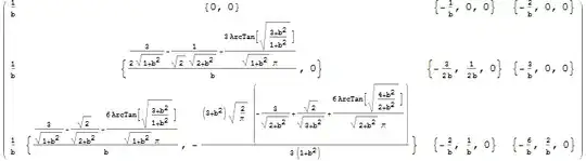
which matches the results given in this answer above.

Note: It is interesting to look at the limit $a\rightarrow -\infty$ of the result. Clearly we have: \begin{eqnarray} \lim\limits_{a\rightarrow -\infty} {\mathfrak J}^{(n)}(a,b) = g_0^{(n)}(b)= \left\{\frac{1}{b},\frac{1}{b},\frac{1}{b},\frac{1}{b},g^{(5)}_0(b),\cdots\right\} \end{eqnarray} for $n=1,\cdots,5$. Here: \begin{eqnarray} &&6 \pi ^2 b \left(b^2+2\right) \sqrt{b^2+3}g_0^{(5)}(b)=\\ &&15 \left(b^2+4\right)^{3/2} \left(\pi -2 \tan ^{-1}\left(\sqrt{\frac{b^2+5}{b^2+3}}\right)\right)-5 \pi \sqrt{b^2+3} \left(b^2 \left(\sqrt{2}-6 \sin ^{-1}\left(\frac{1}{\sqrt{3}}\right)\right)+4 \left(\sqrt{2}-3 \sin ^{-1}\left(\frac{1}{\sqrt{3}}\right)\right)\right) \end{eqnarray} Now, if we expand the quantity above in a Taylor series in powers of $1/b$ we get: \begin{eqnarray} g_0^{(5)}(b)= 1.00232 \frac{1}{b} - 0.00884816 \frac{1}{b^3} + 0.0402526 \frac{1}{b^5}+O(\frac{1}{b^7}) \end{eqnarray} and as such we see that the quantity in question is still quite close to $1/b$. On the other hand if we were to compute that limit naively from definition by exchanging the limit and the integration we would have obtained: \begin{eqnarray} &&\lim\limits_{a\rightarrow -\infty} {\mathfrak J}^{(n)}(a,b)= \lim\limits_{a\rightarrow -\infty}\int\limits_{\mathbb R} [\Phi(\frac{x-a}{b})]^n \cdot \phi(x) \frac{dx}{b} \overbrace{=}^{?}\\ && \int\limits_{\mathbb R} \lim\limits_{a\rightarrow -\infty}[\Phi(\frac{x-a}{b})]^n \cdot \phi(x) \frac{dx}{b} = \int\limits_{\mathbb R} \phi(x) \frac{dx}{b} = \frac{1}{b} \end{eqnarray}

As we can see swapping of the limit and the integration is not always allowed and in fact for $n\ge 5$ it leads to a slightly different result.

Answer 2

If we assume that $b$ is large, we can try the Laplace method see http://en.wikipedia.org/wiki/Laplace%27s_method look under "Other formulations". This assumes that the integrand is maximal at $-a/b$ and decays fast around this point. This gives $$ \int \Phi^n(x)\phi(bx+a) dx \approx \Phi^n(-a/b)\int \phi(bx+a) dx=$$ $$\Phi^n(-a/b) \frac{1}{b}$$ This is now the quick and dirty proposal. If it doesn't help, (please some information about the context), maybe one can try Laplace's method in some other way, i.e. with $n$ as large parameter.

Answer 3

Following the methods explained in the post integrating-pdf-times-cdf-squared (restates the integral in terms of probability arguments) and redefining the same integral we obtain, \begin{eqnarray} \int_{-\infty}^{\infty}\Phi(x)^{n}\phi(a+bx)dx&=&\frac{1}{b}\int_{-\infty}^{\infty}\Phi\left(\frac{y-a}{b}\right)^{n}\phi(y)dy\\&=&\frac{1}{b}P\left(z_{1}\leq \frac{y-a}{b},z_{2}\leq \frac{y-a}{b},z_{3}\leq \frac{y-a}{b}....z_{n}\leq \frac{y-a}{b}\right)\\&=&\frac{1}{b}P\left(bz_{1}-y\leq -a,bz_{2}-y\leq -a,bz_{3}-y\leq -a....bz_{n}-y\leq -a\right)\\&=& \frac{1}{b}\mathcal{MVN}\left(x=\{-a,-a,-a...\},\mu=\{0,0,0...\},\Sigma=\begin{bmatrix}b^{2}+1 & 1 & 1&...\\1&1&b^{2}+1&1&...\\1&1&1&b^{2}+1&1... \end{bmatrix} \right) \end{eqnarray} where $\mathcal{MVN}$ is multivariatenormal distribution CDF. An R-based quick application for a=1,b=1, n=3 and a=1,b=2,n=4 shows that indeed the integral in question can be computed using this solution, we can observe this from coinciding results of numerical integral using the definition and the multivariate normal CDF. The only needed effort is to define the covariance matrix.

 sg<-function(a,b,x){pnorm(x)^3*dnorm(a+b*x)}
 integrate(sg,-Inf,Inf,a=1.,b=1.)
0.06832488 with absolute error < 4.9e-07
pmnorm(x = c(-1.,-1.,-1),mean = rep(0.,3),varcov = matrix(c(2,1.,1.,1.,2,1.,1,1,2),ncol=3,byrow=T))
[1] 0.06832488
sg<-function(a,b,x){pnorm(x)^4dnorm(a+bx)}
> integrate(sg,-Inf,Inf,a=1.,b=2.)
0.01677928 with absolute error < 3.3e-05
pmnorm(x = c(-1.,-1.,-1,-1),mean = rep(0.,4),varcov = matrix(c(5,1.,1.,1.,1,5,1.,1,1,1,5,1,1,1,1,5),ncol=4,byrow=T))/2.
[1] 0.0167786